Extended Kalman Filter Implementation for Constant Turn Rate and Acceleration(CTRA) Vehicle Model in Python.
- 扩展的卡尔曼滤波器,其状态转移和观察模型不需要一定是状态的线性函数,而是状态的可微函数;
-
-
- 这里,
和
是过程和观测噪声,假设它们均为零均值多变量高斯噪声,协方差矩阵分别记为
和
-
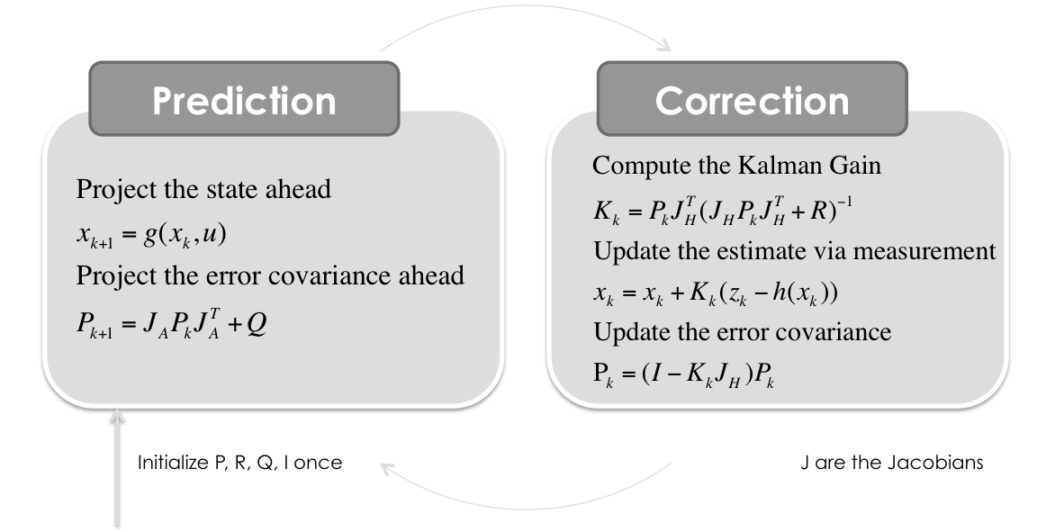
函数可以根据先前估计值
来计算现在状态的估计值,
函数可以从预测状态中计算出预测测量值。但是,
和
不可以直接应用于协方差矩阵,而是通过一个偏微分矩阵(雅克比矩阵
)
- 在每一个时间增量步,通过当前预估状态评估雅克比行列式,这些Matrix被用在卡尔曼滤波器等式中,该过程基本上使目前估计值周围的非线性函数线性化。
- 情境:Situation coverd...
- 你有一个速度传感器,测量车辆速度(
)以及车头的方向(
)以及一个偏航(Yaw)角速度传感器(
),这些与一个GPS传感器的坐标信息(x&y)进行融合。
- 你有一个速度传感器,测量车辆速度(
必要工具包
状态向量——常转速以及加速度车辆模型(Constant Turn Rate and Acceleration Vehicle Model CTRA)


- 首先将各个状态变量定义好
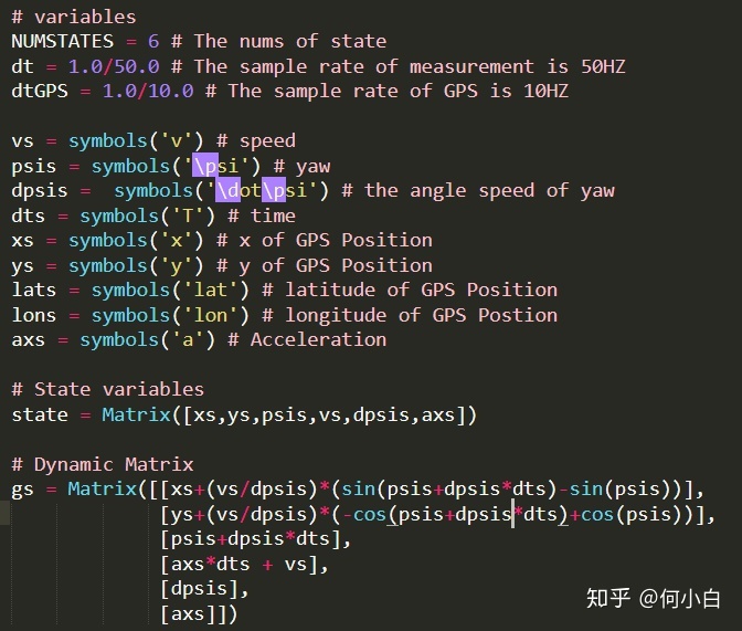
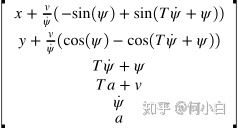
- 可以得到:状态向量与动力学矩阵的字符表达(很简单,可以自己推一下):

- 同时,利用如下语句,可以得到该模型的雅克比矩阵


- 这个雅克比矩阵,在每一个过滤器step进行计算,因为其包含了各个状态变量;
- P.S. A.topython 和 .to_c 或者.to_matlab可以生成相应格式的代码;
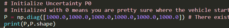
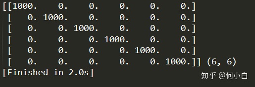
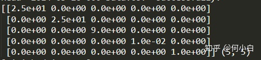
初始化不确定矩阵
- 注意,如果以0来初始这个矩阵
,这就代表着,你非常确定该车辆的启动位置;
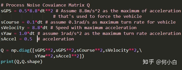
处理噪声协方差矩阵Q
- 按照论文里面进行模型的处理,该论文指出,状态不确定性模型激发线性系统的扰动,从概念上来说,其评估了当系统在给定时间段内开环运行时会有多糟糕。
读取测量数据

其中注意,对于course要做如下处理:course = -course + 90°,原因很简单,航向为0°,意味着这两车在成向整备方向行驶,90°意味着这辆车正在沿者正东方向行驶。后面的计算,我们 规定正东方向是0°,而正北方向是90°,这需要统一(参考坐标系)。
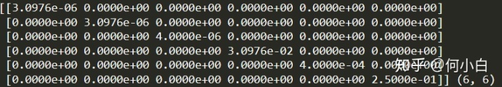
测量函数H
- 矩阵
函数H可以被用来通过预测状态值来计算预测测量值。
是测量函数H关于各个状态变量的雅克比矩阵,
- 如果有可用的GPS测量值,下面的函数将状态变量映射到测量值。
- 如果没有可用的GPS测量值,简单的设置
为0矩阵。
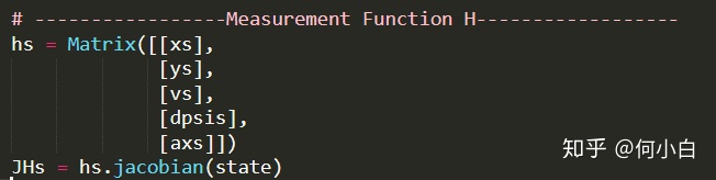

测量噪声协方差矩阵R
- 实际使用时,不确定性估计采用状态估计和测量的相对权重的重要性大小,也就是说R大,则状态估计值占比会比较大,R小则观测值(测量值)的占比较大,所以,不确定性估计是否绝对正确不是那么重要,因为其在每一种模型中的占比相对一致。
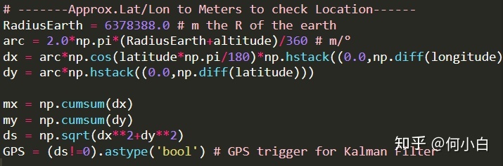
将经纬度信息转化为m为单位的坐标信息
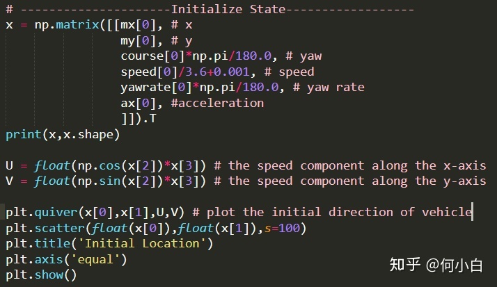
初始化State
- 利用下段代码,就可以初始化车辆的初始坐标以及方向;

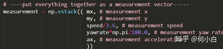
将所有观测量几何成一个vector
进行EKF扩展卡尔曼滤波算法
- 按照Dynamic Equation对每个状态变量进行预测
- 计算Jacobin矩阵
- 预测误差协方差
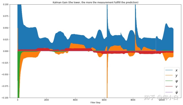
- 计算卡尔曼增益K
- 根据观测值来更新预测值
- 更新误差协方差矩阵P
for 
Plot结果
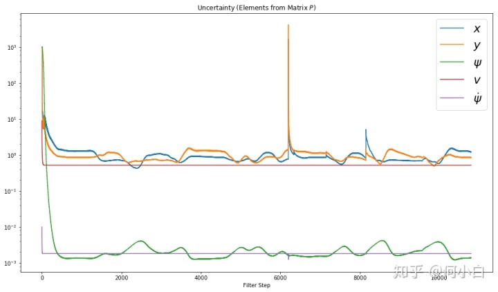
- 不确定性
- 卡尔曼增益
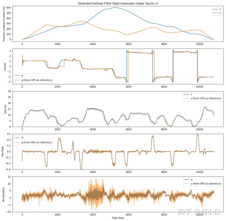
- 各个状态变量的跟踪情况
- 位置X/Y的跟踪详情
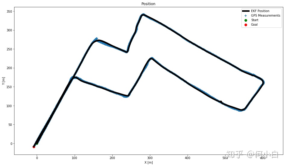
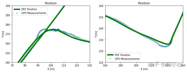
通过使用EKF,达到很好的预测跟踪效果~